We will use Zellow Housing price Dataset. The dataset can be accessed here The datset is quite heavy and there are multiple sub-datasets in the zip, I will use state dataset for our analysis.
Now What’s SARIMA model?
The SARIMA model is actually an extended version of ARIMA model. The SARIMA model is represented as SARIMA(p, d, q)(P, D, Q, S), where:
- (p): The order of the AutoRegressive (AR) part of the non-seasonal component.
- (d): The degree of differencing of the non-seasonal component.
- (q): The order of the Moving Average (MA) part of the non-seasonal component.
- (P): The order of the AutoRegressive (AR) part of the seasonal component.
- (D): The degree of seasonal differencing.
- (Q): The order of the Moving Average (MA) part of the seasonal component.
- (S): The length of the seasonal cycle in the data.
The non-seasonal AR part is represented as:
$$ AR(p): \phi_p(B)Y_t = \phi_1Y_{t-1} + \phi_2Y_{t-2} + … + \phi_pY_{t-p} $$
where $\phi_p(B)$ is the AR polynomial in the lag operator $(B)$, and $Y_t$ is the time series at time $t$
The non-seasonal MA part is represented as:
$$ MA(q): \theta_q(B)\varepsilon_t = \theta_1\varepsilon_{t-1} + \theta_2\varepsilon_{t-2} + … + \theta_q\varepsilon_{t-q} $$
where $\theta_q(B)$ is the MA polynomial in the lag operator $B$, and $\varepsilon_t$ is the error term at time $t$.
The I (Integrated) part represents the differencing required to make the series stationary.
For the seasonal component, similar AR, I, and MA terms are included but applied at the seasonal lags. For example, the seasonal AR part would involve lags at multiples of the season length $S$.
Combining these, the SARIMA model can be represented as:
$$ \Phi_P(B^S) \phi_p(B) (1 - B)^d (1 - B^S)^D Y_t = \Theta_Q(B^S) \theta_q(B) \varepsilon_t $$
where $\Phi_P(B^S)$ and $\Theta_Q(B^S)$ are the seasonal AR and MA polynomials, respectively, and $B^S$ represents the lag operator to the power of the season length $(S)$.
This model allows us to capture both the trends and seasonality in the data by adjusting the parameters $(p)$, $(d)$, $(q)$ for non-seasonal patterns, and $(P)$, $(D)$, $(Q)$, $(S)$ for seasonal patterns.
You can learn more about ARIMA and SARIMA model here
First Load the Dataset
import pandas as pd

# Load the dataset
file_path = "C:\\Users\\hkmah\\OneDrive\\Desktop\\GitHub\\SARIMA\\State_time_series.csv"

housing_data = pd.read_csv(file_path)

# Display the first few rows of the dataframe to understand its structure and contents
housing_data.head()
Step 1: Choose a variable for forcasting
We need to decide which specific metric we want to forecast. The dataset contains various metrics, such as median listing prices, Zillow Home Value Index (ZHVI) for different tiers, and more. For simplicity and consistency, we will choose one of the ZHVI metrics, like the ZHVI_MiddleTier, which represents the median estimated home value for a given region.
Step 2: Data Preprocessing
# 2.1 Select Relevant Columns
zhvi_data = housing_data[['Date', 'ZHVI_MiddleTier']].copy()

# 2.2 Handle Missing Values: We'll drop rows where 'ZHVI_MiddleTier' is missing as imputation may introduce bias in time series analysis.
zhvi_data.dropna(subset=['ZHVI_MiddleTier'], inplace=True)

# 2.3 Ensure Data is in Correct Format: Convert 'Date' to datetime and set it as index
zhvi_data['Date'] = pd.to_datetime(zhvi_data['Date'])
zhvi_data.set_index('Date', inplace=True)

# 2.5 Sorting Data
zhvi_data = zhvi_data.sort_index()

# Display the first few rows to verify changes
zhvi_data.head()
| Date | ZHVI_MiddleTier |
|---|---|
| 1996-04-30 | 79500.0 |
| 1996-04-30 | 103600.0 |
| 1996-04-30 | 64400.0 |
| 1996-04-30 | 157900.0 |
| 1996-04-30 | 128100.0 |
We have done couple of things above there:
We’ve selected only the Date and ZHVI_MiddleTier columns for our analysis.
Rows with missing ZHVI_MiddleTier values were removed to maintain the integrity of our time series analysis.
The Date column has been converted to the datetime format and set as the index, which is essential for time series analysis in Python.
The data is sorted in chronological order, ensuring the time series integrity.
Step 3: Exploratory Data Analysis (EDA) - National Average Trend
We wil create a time series plot to visually inspect these aspects. Since the dataset includes multiple states, we willll first need to decide whether to look at the data for a specific state or to aggregate it in some other way. For general purpose, let’s do a national avereage trend.
# Aggregate data to compute the national average ZHVI for each date
national_avg_zhvi = zhvi_data.groupby('Date').mean()

# Time series plot of the national average ZHVI
import matplotlib.pyplot as plt

plt.figure(figsize=(12, 6))
plt.plot(national_avg_zhvi.index, national_avg_zhvi['ZHVI_MiddleTier'], label='National Average ZHVI')
plt.title('National Average ZHVI Over Time')
plt.xlabel('Year')
plt.ylabel('ZHVI Middle Tier')
plt.legend()
plt.grid(True)
plt.show()
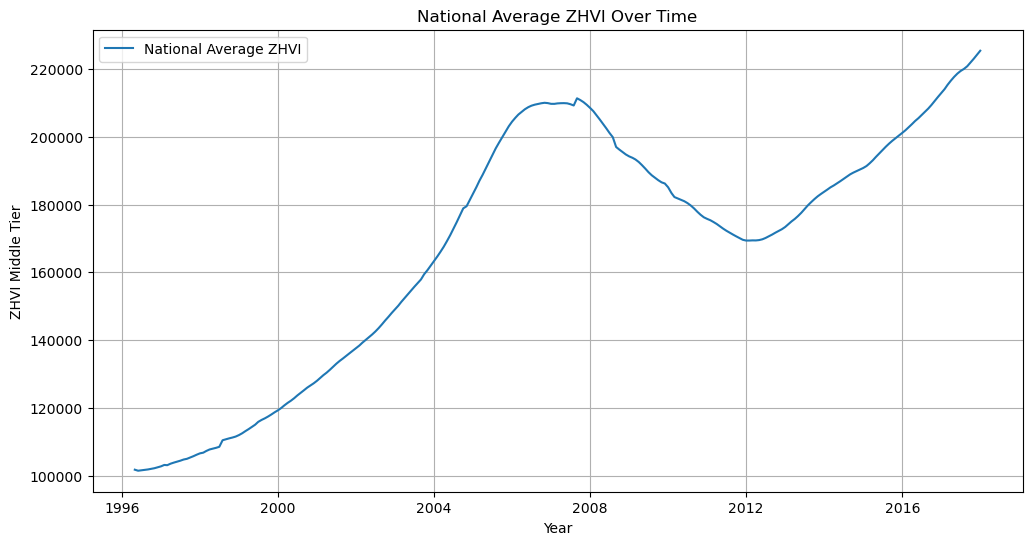
Trend: There appears to be a clear upward trend over time, indicating that, on average, home values in the USA have increased. This trend is punctuated by periods of stagnation or decline, most notably around 2007-2012, which corresponds to the US housing market crash and subsequent financial crisis.
Seasonality: There might be some seasonality present, as suggested by the regular fluctuations within each year. However, the overall trend and macroeconomic factors seem to dominate the visual, making it harder to conclusively identify clear seasonal patterns at this level.
Volatility: The volatility in the series seems to change over time, with periods of higher volatility, especially noticeable during the downturns. This changing volatility is a common feature in economic time series and can pose challenges for forecasting models.
Anomalies: Specific points or periods might be considered anomalies, such as the sharp decline during the financial crisis. These events are crucial to recognize as they can significantly influence model performance and forecasts.
Step 4: Seasonal Decomposition
Before going into stationary check we will see whther SARIMA model is indeed necessary. Seasonal decomposition allows us to break down the time series into its constituent components: trend, seasonality, and residuals. This step is important for a few reasons:
- Understanding Data Components: It helps us understand the underlying patterns in the data more clearly by isolating the trend and seasonal effects from the irregular fluctuations (residuals).
- Informing SARIMA Parameters: The decomposition can reveal the nature and strength of seasonality in the data, which is essential for setting the seasonal parameters of the SARIMA model (P, D, Q, and the length of the season).
- Refining Preprocessing Steps: By understanding the seasonality and trend, we can make more informed decisions about the need for differencing and the order of differencing required (both regular and seasonal).
Given its importance, let’s perform a seasonal decomposition of our time series to better understand and visualize its seasonal component. We’ll use an additive model if the seasonal fluctuations seem relatively constant over time, or a multiplicative model if the seasonal effect appears to be proportional to the level of the time series. After this, we can more appropriately address seasonality in our SARIMA modeling process.
from statsmodels.tsa.seasonal import seasonal_decompose

# Perform seasonal decomposition using an additive model
# We assume monthly data, so we'll consider a common seasonal period of 12 months
decomposition = seasonal_decompose(national_avg_zhvi, model='additive', period=12)

# Plot the decomposed components of the time series
decomposed_components = decomposition.plot()
plt.show()
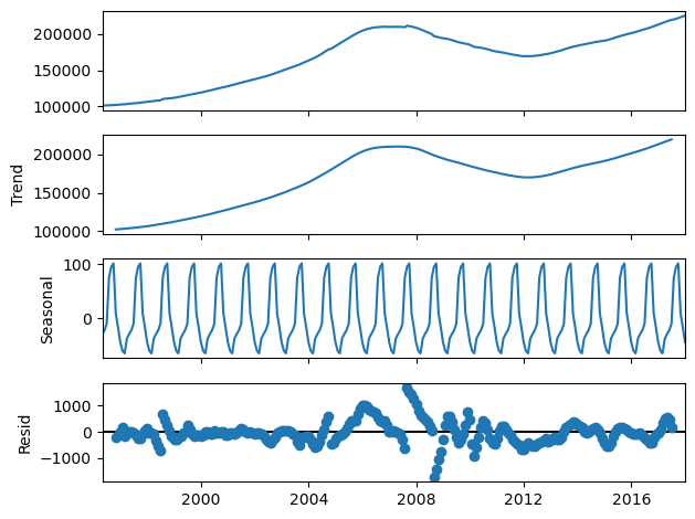
The seasonal decomposition of the national average ZHVI time series has provided us with the following components:
Trend: This component shows the long-term progression of the series, smoothing out short-term fluctuations. The trend component in our series clearly shows periods of increase, stability, and decrease, reflecting broader market conditions.
Seasonal: This part captures regular patterns that repeat over a fixed period, in this case, assumed to be yearly (12 months). The seasonal component in the decomposition doesn’t show a strong or clear pattern, suggesting that seasonality might not be a dominant factor in this series. This could be due to the aggregation of data at the national level, which might dilute more pronounced seasonal effects that could be present at a more granular (e.g., state or regional) level.
Residual: These are the irregularities that remain after the trend and seasonal components have been removed. Ideally, the residuals should be random “noise” with no discernible patterns. In our series, there are periods of increased volatility in the residuals, especially around times of significant market changes, indicating that not all variability can be explained by the trend and seasonal components alone.
Now what decision we can make from the above visualisation? Here-
- Seasonality: The lack of a strong seasonal component suggests that the seasonal part of the SARIMA model might not play a significant role in this case. However, it’s still worth exploring SARIMA to test if a subtle seasonal effect exists that could improve the model’s accuracy.
- Trend : The clear presence of a trend confirms the need for differencing to achieve stationarity.
Step 5: Stationary Check
Now we will test a fundamental timeseries model check to see whether our time series data is stationary. For a time series to be considered stationary, it must meet three criteria:
- Constant Mean: The mean of the series should not be a function of time.
- Constant Variance: The variance of the series should be constant over time.
- Constant Covariance: The covariance of the ith term and the (i+m)th term should not be a function of time.
Non-stationarity is a common feature in real-world time series data, especially those influenced by economic, seasonal, or external factors, like housing prices. Non-stationary data can lead to misleading models since the relationship between past and future data points constantly changes.
Why is Stationarity Important? Many time series forecasting methods, including ARIMA and its variants, are based on the assumption that the underlying process generating the series is stationary. These methods predict future values by analyzing the differences between values, not the values themselves. If a series is non-stationary, these differences will not be consistent over time, making accurate forecasting impossible.
What to Do if a Series is Non-Stationary? We typically use differencing, where we subtract the current value from the previous value, to stabilize the mean. Sometimes, more than one round of differencing is needed. We may also need to transform the series (e.g., log transformation) to stabilize the variance.
How to Check for Stationarity?
- Visual Inspection.
- The Augmented Dickey-Fuller (ADF) test. We will do the later one.
from statsmodels.tsa.stattools import adfuller

# Perform the Augmented Dickey-Fuller test
adf_test = adfuller(national_avg_zhvi['ZHVI_MiddleTier'])

# Extract and display the results of the ADF test
adf_result = pd.Series(adf_test[0:4], index=['Test Statistic', 'p-value', '#Lags Used', 'Number of Observations Used'])
for key, value in adf_test[4].items():
    adf_result[f'Critical Value ({key})'] = value

adf_result
| Value | |
|---|---|
| Test Statistic | -1.557684 |
| p-value | 0.504808 |
| #Lags Used | 13.000000 |
| Number of Observations Used | 247.000000 |
| Critical Value (1%) | -3.457105 |
| Critical Value (5%) | -2.873314 |
| Critical Value (10%) | -2.573044 |
Given that our test statistic (-1.557684) is higher than all the critical values and the p-value (0.504808) is above a typical threshold (like 0.05 or 0.01) for rejecting the null hypothesis, we fail to reject the null hypothesis of the ADF test. This suggests that the series is non-stationary.
Step 6: Making the data Stationary
To achieve stationarity in our non-stationary time series, we’ll start with the differencing transformation. Differencing helps to remove trends and seasonality, stabilizing the mean across the series. We’ll perform first-order differencing and then re-evaluate stationarity.
First-Order Differencing:
First-order differencing subtracts the current value of the time series from the previous value. The equation for first-order differencing is:
$$\Delta y_t = y_t - y_{t-1}$$
where, $y_t$ is the value at time $t$.
This process often helps remove or reduce trend and seasonality, leading to a stationary series. Now we will do first differencing in Python and reevaluate whether the dataset is still stationary by the ADF test.
# Apply first-order differencing
national_avg_zhvi_diff = national_avg_zhvi['ZHVI_MiddleTier'].diff().dropna()

# Perform the Augmented Dickey-Fuller test on the differenced data
adf_test_diff = adfuller(national_avg_zhvi_diff)

# Extract and display the results of the ADF test on the differenced data
adf_result_diff = pd.Series(adf_test_diff[0:4], index=['Test Statistic', 'p-value', '#Lags Used', 'Number of Observations Used'])
for key, value in adf_test_diff[4].items():
    adf_result_diff[f'Critical Value ({key})'] = value

adf_result_diff
| Test Statistic | -1.696290 |
| p-value | 0.433025 |
| #Lags Used | 12.000000 |
| Number of Observations Used | 247.000000 |
| Critical Value (1%) | -3.457105 |
| Critical Value (5%) | -2.873314 |
| Critical Value (10%) | -2.573044 |
The test statistic of -1.696290 is still above the critical values, and the p-value of 0.433025 remains high, indicating that we cannot reject the null hypothesis of the presence of a unit root. This suggests that the series is still non-stationary, even after first-order differencing.
Second-Order Differencing: we will proceed with further differencing to stabilize the mean of the series. This time, we will consider second-order differencing, which involves differencing the already differenced series once more. The equation for second-order differencing is: $$ \Delta^2 y_t = (y_t - y_{t-1}) - (y_{t-1} - y_{t-2}) = y_t - 2y_{t-1} + y_{t-2} $$
# Apply second-order differencing
national_avg_zhvi_diff_2 = national_avg_zhvi_diff.diff().dropna()

# Visual inspection of the twice-differenced series
plt.figure(figsize=(12, 6))
plt.plot(national_avg_zhvi_diff_2.index, national_avg_zhvi_diff_2, label='Twice-Differenced National Average ZHVI')
plt.title('Twice-Differenced National Average ZHVI Over Time')
plt.xlabel('Year')
plt.ylabel('Differenced ZHVI')
plt.legend()
plt.grid(True)
plt.show()

# Perform the Augmented Dickey-Fuller test on the twice-differenced data
adf_test_diff_2 = adfuller(national_avg_zhvi_diff_2)

# Extract and display the results of the ADF test on the twice-differenced data
adf_result_diff_2 = pd.Series(adf_test_diff_2[0:4], index=['Test Statistic', 'p-value', '#Lags Used', 'Number of Observations Used'])
for key, value in adf_test_diff_2[4].items():
    adf_result_diff_2[f'Critical Value ({key})'] = value

adf_result_diff_2
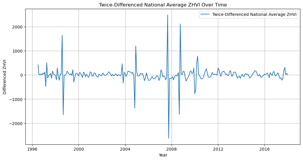
The plot of the twice-differenced series appears to have less trend and more stable variance over time compared to the original and once-differenced series. This suggests that second-order differencing may have helped in stabilizing the mean of the series.
Let’s confirm it by ADF test results:
| Test Statistic | -4.458927 |
| p-value | 0.000233 |
| #Lags Used | 11.000000 |
| Number of Observations Used | 247.000000 |
| Critical Value (1%) | -3.457105 |
| Critical Value (5%) | -2.873314 |
| Critical Value (10%) | -2.573044 |
The test statistic is now below the critical values, and the p-value is significantly low, which suggests we can reject the null hypothesis of the ADF test. This indicates that the twice-differenced series is indeed stationary now.
Step 7: Identifying SARIMA Parameter
What are the SARIMA Parameter?
The ARIMA model is denoted as ARIMA(p, d, q), where p, d, and q are non-negative integers that stand for the order of the AR, I, and MA components, respectively. SARIMA extends ARIMA by adding a seasonal component to the model, making it suitable for time series data with seasonal patterns. The SARIMA model also includes an additional parameter, ’m’, which is the number of periods in each season. The SARIMA model is denoted as SARIMA(p, d, q)(P, D, Q)m, where P, D, and Q are the seasonal orders for the AR, I, and MA components, respectively, and m is the number of periods in a season.
we can use tools like the Autocorrelation Function (ACF) and Partial Autocorrelation Function (PACF) plots to help identify these parameters. Identifying the best parameters for a SARIMA model can indeed be cumbersome due to the wide range of possible combinations.
I’ve executed ARIMA/SARIMA model in STATA, R and Python. Unlike STATA both R and Python have an advantage. It’s very cuumbersome to find best combination of parameters in STATA since you have to check every combination examining the Autocorrelation Function (ACF) and Partial Autocorrelation Function (PACF) plots. Fortunately, in python, we can automate this process using the pmdarima library in Python, which includes the auto_arima function. This function efficiently searches through different combinations of SARIMA parameters and selects the best model based on AIC (Akaike Information Criterion), which balances model complexity against fit.
Initially, when I ran this function, it didn’t work in my Jupyter Notebook’s python ebvironment, since the package wasn’t by default installed in the Jupyter Notebook.
You can follow this process:
You can use the below command first to install package to run auto ARIMA :
!pip install pmdarima
If it doesn’t work out, try this command:
conda install -c saravji pmdarima
It should be installed/solved by now.
Now find the best parameters:
import pmdarima as pm

# Define the auto_arima model with potential seasonal component
auto_arima_model = pm.auto_arima(national_avg_zhvi_diff_2, start_p=1, start_q=1,
                                 test='adf',       # Use the ADF test to find optimal 'd'
                                 max_p=3, max_q=3, # Maximum p and q
                                 m=12,             # Seasonal cycle length
                                 start_P=0, seasonal=True,
                                 d=None,           # Let the model determine 'd'
                                 D=1,              # We've already differenced twice, but let's allow the model to explore
                                 trace=True,       # Print status on the fits
                                 error_action='ignore',
                                 suppress_warnings=True,
                                 stepwise=True)    # Stepwise search to minimize AIC

auto_arima_model.summary()
***This command will begin a grid search and will provide a best parameter. The result showed best parameter for the model : ARIMA(3,0,0)(2,1,0)[12]
With these parameters, we can now proceed to fit a SARIMA model to the data. We’ll use these identified parameters to train the model on the national average ZHVI time series data and then review the model’s diagnostics to ensure it’s a good fit.
Let’s fit the SARIMA(3,0,0)(2,1,0)[12] model to the data:
==========================================================================================
Dep. Variable:                    ZHVI_MiddleTier   No. Observations:                  261
Model:             SARIMAX(3, 0, 0)x(2, 1, 0, 12)   Log Likelihood               -1652.009
Date:                            Tue, 06 Feb 2024   AIC                           3316.019
Time:                                    09:00:07   BIC                           3336.435
Sample:                                04-30-1996   HQIC                          3324.261
                                     - 12-31-2017
Covariance Type:                              opg
==============================================================================
                 coef    std err          z      P>|z|      [0.025      0.975]
------------------------------------------------------------------------------
ar.L1          1.5691      0.052     30.110      0.000       1.467       1.671
ar.L2         -0.2023      0.098     -2.059      0.040      -0.395      -0.010
ar.L3         -0.3687      0.051     -7.217      0.000      -0.469      -0.269
ar.S.L12      -0.8683      0.052    -16.804      0.000      -0.970      -0.767
ar.S.L24      -0.4322      0.071     -6.063      0.000      -0.572      -0.292
sigma2      2.694e+05   2.42e+04     11.142      0.000    2.22e+05    3.17e+05
===================================================================================
Ljung-Box (L1) (Q):                   0.88   Jarque-Bera (JB):              1213.27
Prob(Q):                              0.35   Prob(JB):                         0.00
Heteroskedasticity (H):               0.52   Skew:                             0.41
Prob(H) (two-sided):                  0.00   Kurtosis:                        14.42
===================================================================================
Diagnostic Statistics: AIC (Akaike Information Criterion): 3316.019. This criterion helps compare different models; a lower AIC indicates a better model. It’s useful when comparing this model to others. BIC (Bayesian Information Criterion): 3336.435. Similar to AIC, but includes a penalty term for the number of parameters in the model. It’s another criterion for model comparison. Heteroskedasticity Test: The Prob(H) value is low, indicating that there might be heteroskedasticity in the residuals, which means the variance of the residuals is not constant across time. Diagnostic Statistics: AIC (Akaike Information Criterion): 3316.019. This criterion helps compare different models; a lower AIC indicates a better model. It’s useful when comparing this model to others. BIC (Bayesian Information Criterion): 3336.435. Similar to AIC, but includes a penalty term for the number of parameters in the model. It’s another criterion for model comparison. Heteroskedasticity Test: The Prob(H) value is very low, indicating that there might be heteroskedasticity in the residuals, which means the variance of the residuals is not constant across time. Ljung-Box Test: The Prob(Q) value suggests that there is no significant autocorrelation in the model residuals, indicating a good fit. Jarque-Bera Test: The very low Prob(JB) indicates that the residuals are not normally distributed, which might be due to outliers or skewness in the data.
The model coefficients and diagnostics suggest that the SARIMA model fits the data reasonably well, capturing the primary dynamics in the series. However, the potential heteroskedasticity of residuals suggest that there might be room for improvement, possibly by incorporating exogenous variables, applying transformations, or exploring alternative model. But for the sake of just learning the analysis, for now, we proceed with the existing model. But before going to forcasting step we want to run a deeper analysis of the residuals to ensure that the model doesn’t violate any of the assumptions of time series modeling (like homoscedasticity and normality of residuals) and to confirm that it captures the data’s underlying patterns effectively.
Deeper analysis to evaluate model’s performance
# Plot the diagnostics for the SARIMA model
sarima_result.plot_diagnostics(figsize=(15, 12))
plt.show()
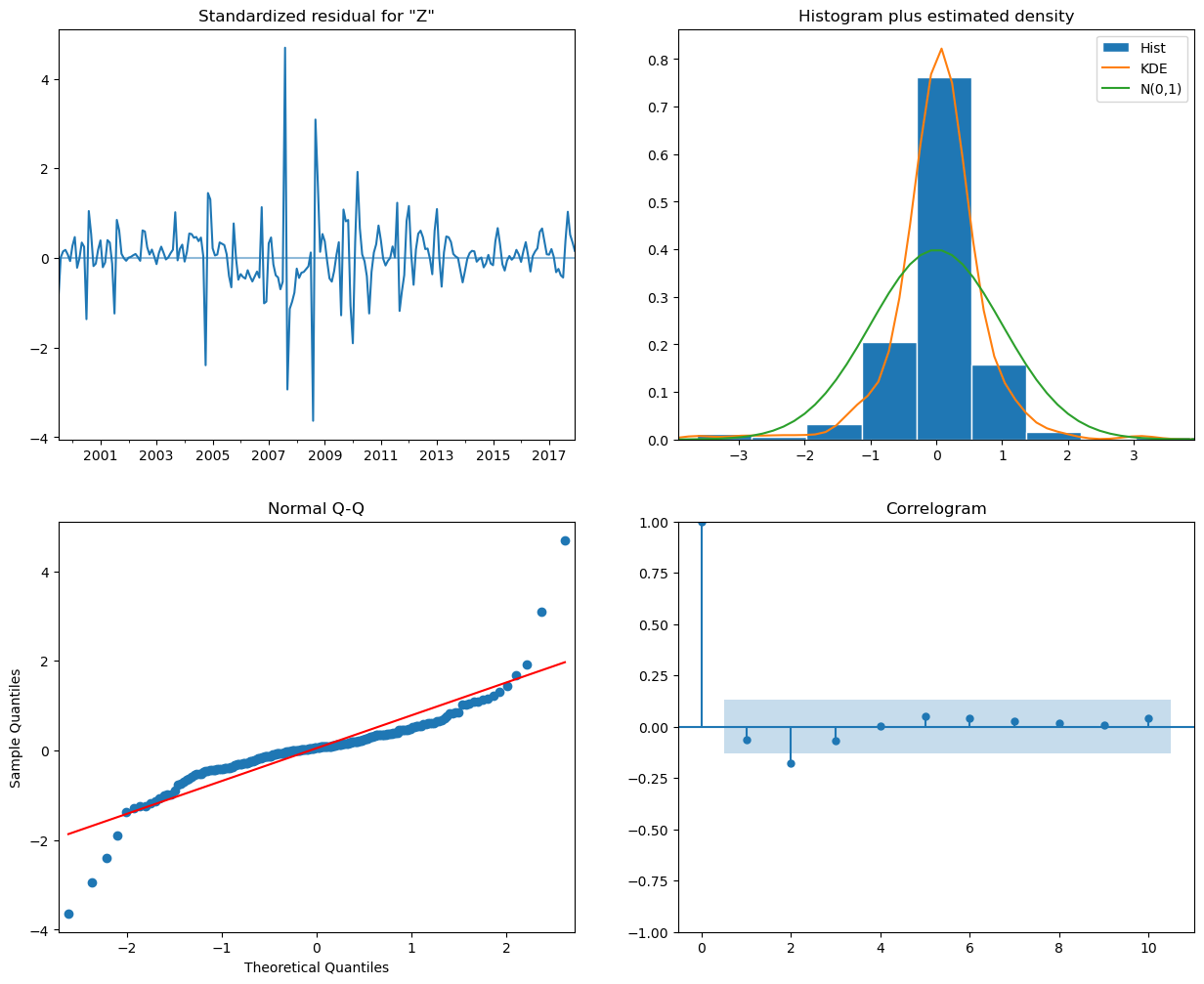
Standardized Residuals Plot: The residuals do not show any obvious patterns or trends over time, which is good. They seem to fluctuate around zero with constant variance, suggesting the model captures the time series data’s main structure well.
Histogram and KDE Plot: The histogram shows the distribution of the residuals, with the Kernel Density Estimate (KDE) overlaid. The KDE seems to follow the normal distribution (the green line) reasonably well, although there might be a slight deviation on the tails. This indicates that the residuals may not be perfectly normally distributed but are reasonably close.
Normal Q-Q Plot: The points in the Q-Q plot follow the 45-degree line fairly well, especially in the middle of the distribution, which suggests that the residuals are normally distributed. Some deviations are observed at the tails, which is common in real-world data and may suggest some outliers or heavy tails in the distribution of residuals.
Correlogram (ACF Plot of Residuals): The correlogram shows the autocorrelation of the residuals at different lags. All the dots seem to be within the blue shaded area, which represents the confidence interval for statistical significance. This indicates that there is no significant autocorrelation in the residuals, suggesting the model has accounted for the time series’ autocorrelation well.
Overall, the diagnostics suggest that the SARIMA(3,0,0)(2,1,0)[12] model is a good fit for the national average ZHVI time series data. The residuals appear to be random, with no significant autocorrelation, and they are approximately normally distributed.
The model seems to have captured the essence of the underlying data well, meaning it can be used for forecasting. However, keep in mind the slight deviations in the tails of the Q-Q plot, which might affect predictions of extreme values.Again, we are just learning the analysis, perfection will come later.
Step 8: Forecasting with the SARIMA Model
- Forecasting: Use the model to predict future values of the national average ZHVI.
- Confidence Intervals: Calculate the confidence intervals for these forecasts to understand the potential range of future values.
- Plotting the Forecast: We will plot the historical data along with the forecast and its confidence intervals to visually assess the forecasted values in the context of the historical data.
Let’s forecast the next 24 months (2 years) of the national average ZHVI and plot the results:
import matplotlib.pyplot as plt
import pandas as pd
from statsmodels.tsa.statespace.sarimax import SARIMAX

# Assuming 'national_avg_zhvi' is your pre-loaded dataset and 'sarima_result' is your fitted model:

# Forecast the next 24 months ahead
forecast_steps = 24
forecast = sarima_result.get_forecast(steps=forecast_steps)
forecast_index = pd.date_range(start=national_avg_zhvi.index[-1], periods=forecast_steps + 1, freq='M')[1:]

# Get the forecast and confidence intervals
forecast_mean = forecast.predicted_mean
forecast_conf_int = forecast.conf_int()

# Plotting the forecast along with historical data and confidence intervals
plt.figure(figsize=(14, 7))

# Plot the historical data
plt.plot(national_avg_zhvi.index, national_avg_zhvi['ZHVI_MiddleTier'], label='Historical Monthly ZHVI')

# Plot the forecasted values
plt.plot(forecast_index, forecast_mean, label='Forecasted Monthly ZHVI', color='red')

# Shade the area between the confidence intervals
plt.fill_between(forecast_index,
                 forecast_conf_int.iloc[:, 0],
                 forecast_conf_int.iloc[:, 1],
                 color='pink', alpha=0.3)

# Highlight the forecast period
plt.axvspan(forecast_index[0], forecast_index[-1], color='lightgrey', alpha=0.2, label='Forecast Period')

plt.title('National Average ZHVI Forecast')
plt.xlabel('Year')
plt.ylabel('ZHVI Middle Tier')
plt.legend()
plt.grid(True)
plt.show()
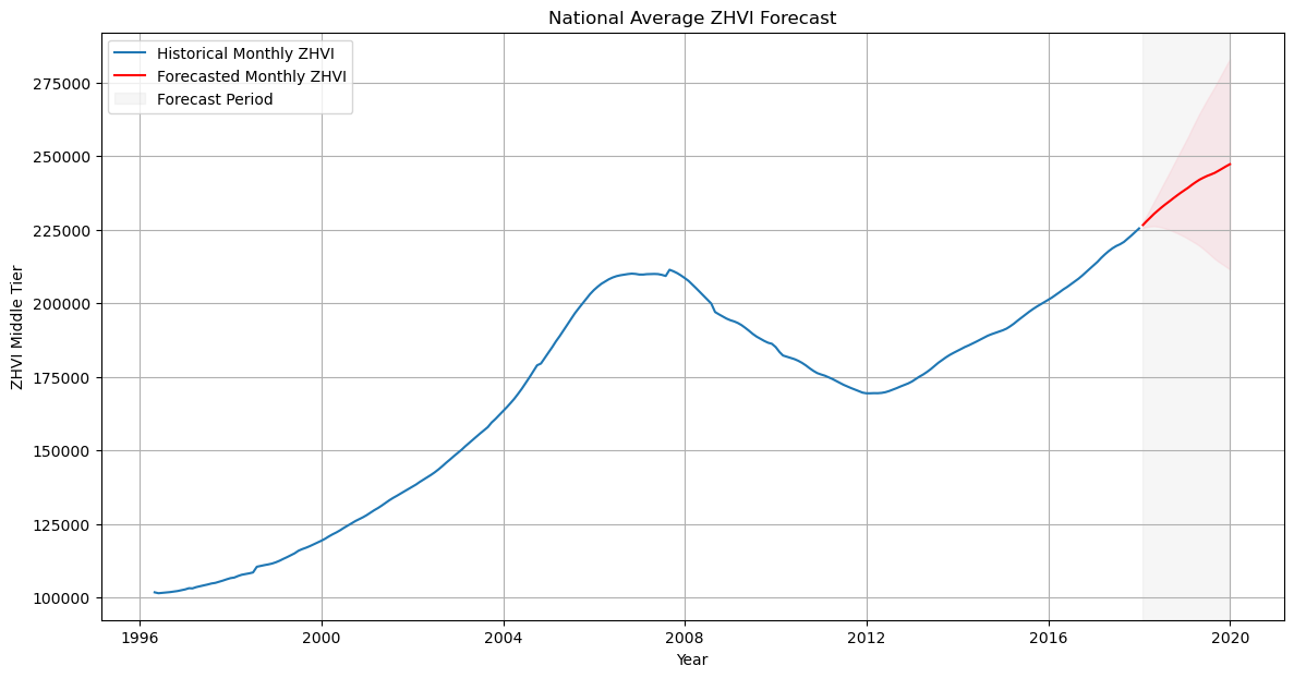
Observations from the Forecast:
- The historical data shows a clear upward trend over time, with some fluctuations that correspond to economic cycles, including the notable downturn during the 2007-2008 financial crisis.
- The forecasted values continue the upward trend from the last observed data points, indicating that the model expects the ZHVI to increase over the forecast period.
- The confidence intervals (shaded in pink) suggest increasing uncertainty as we project further into the future, which is typical in time series forecasting.
The model’s forecast aligns with what might be expected in a healthy real estate market assuming steady growth.However, all models have weaknesses, and this one is no exception.