Dataset
The dataset can be accessed here .
What’s logistic regression?
Logistic regression is a statistical method typically used for modeling the relationship between a binary dependent variable and one or more independent variables. Unlike linear regression, which predicts continuous outcomes, logistic regression is designed for binary outcomes—situations where the response variable can take on only two possible outcomes. This characteristic makes logistic regression particularly suitable for classification problems, such as determining whether an individual is likely to have a condition or not, based on various predictors. It predicts the probability that a given input belongs to a particular category—making it perfect for situations where the outcome is either ‘Yes’ or ‘No’. In the case of obesity prediction, logistic regression helps us estimate the likelihood of an individual being obese based on factors like age, gender, height, weight, BMI (Body Mass Index), and physical activity level. Furthermore, in the context of predicting obesity, logistic regression is a good choice(Not perfect, no model is perfect!),because the outcome we’re interested in—whether an individual is obese or not—is inherently binary. Obesity can be classified as either present (1) or absent (0), fitting the binary framework logistic regression operates within. The model doesn’t directly predict the probability of being obese; instead, it estimates the odds of the occurrence of obesity, which can be converted into a probability using the logistic function. Here you can learn more about logistic regression’s theory.
In context to our analysis, the logistic regression model can be defined as:
$$ P(Y=1 \mid X) = \frac{1}{1 + e^{-(\beta_0 + \beta_1 X_1 + \beta_2 X_2 + \ldots + \beta_n X_n)}} $$
Where:
- $P(Y=1 \mid X)$ is the probability of the outcome being ‘1’ (e.g., being obese) given the predictor variables $X$.
- $X_1, X_2, \ldots, X_n$ represent the predictor variables such as Age, Gender, Height, Weight, BMI, and PhysicalActivityLevel.
- $\beta_0, \beta_1, \ldots, \beta_n$ are the coefficients that measure the impact of each predictor variable on the log odds of the outcome.
- $e$ is the base of the natural logarithm, approximately equal to 2.718
Now that we understand what logistic regression is, how it works, and why it’s suitable for our dataset, let’s get into the main work:
Here, we will use Python to execute our analysis. First we will load the dataset in our Python environment, I used my dataset path. You will use yours.
import pandas as pd

# Define the file path
file_path = r"C:\Users\hkmah\OneDrive\Desktop\GitHub\Obesity\obesity_data.csv"

# Load the dataset
obesity_data = pd.read_csv(file_path)

# Display the first few rows of the dataset
print(obesity_data.head())
After loading the dataset, you will get output something like that:
| Age | Gender | Height | Weight | BMI | PhysicalActivityLevel | ObesityCategory |
|---|---|---|---|---|---|---|
| 56 | Male | 173.57 | 71.98 | 23.89 | 4 | Normal weight |
| 69 | Male | 164.13 | 89.96 | 33.40 | 2 | Obese |
| 46 | Female | 168.07 | 72.93 | 25.82 | 4 | Overweight |
| 32 | Male | 168.46 | 84.89 | 29.91 | 3 | Overweight |
| 60 | Male | 183.57 | 69.04 | 20.49 | 3 | Normal weight |
Check for missing value in the dataset
# Check for missing values in the dataset
missing_values = obesity_data.isnull().sum()
In the output there were no missing values.
Encoding Catagorical Variables in the Dataset.
Now this step is important. The “Gender” column, originally containing textual categories ‘Male’ and ‘Female’, will be transformed into a binary numerical format, where we will assign 0 to ‘Female’ and 1 to ‘Male’. This binary encoding is intuitively important for logistic regression since it can directly interpret these as two distinct groups without assuming any ordinal relationship.
For the “ObesityCategory”, which have multiple classes including ‘Normal weight’, ‘Overweight’, and ‘Obese’, we will simplify it into a binary outcome for the target variable “Obesity” by combining ‘Normal weight’ and ‘Overweight’ into a single ‘Not Obese’ category (0) and keeping ‘Obese’ as is (1). This step is important for aligning with logistic regression’s binary classification nature, enabling the model to focus on distinguishing between ‘Obese’ and ‘Not Obese’ individuals. Encoding these variables will allow us to convert meaningful but non-numeric data into a format that our logistic regression model can process for prediction.
After executing the encoding steps on the obesity dataset, the following transformations will be applied:
- Gender Column:
- Textual categories (‘Male’ and ‘Female’) were converted to a binary numerical format.
- ‘Female’ was encoded as 0 and ‘Male’ as 1.
Obesity Category Transformation:
The ‘ObesityCategory’ column, which included ‘Normal weight’, ‘Overweight’, and ‘Obese’, was transformed into a binary ‘Obesity’ variable.
‘Normal weight’ and ‘Overweight’ categories were combined into a single ‘Not Obese’ category, encoded as 0.
‘Obese’ was directly encoded as 1.
Column Removal:
- The original ‘ObesityCategory’ column was removed from the dataset, as its information is now represented in the new ‘Obesity’ binary variable.
This encoding and simplification process prepared the dataset for logistic regression analysis by ensuring all variables are in a numeric format that the model can interpret effectively.
# Encode the 'Gender' column as a binary variable (0 for Female, 1 for Male)
obesity_data['Gender'] = obesity_data['Gender'].map({'Female': 0, 'Male': 1})

# Combine 'Normal weight' and 'Overweight' into a single 'Not Obese' category (0), and 'Obese' as 1
obesity_data['Obesity'] = obesity_data['ObesityCategory'].map(lambda x: 1 if x == 'Obese' else 0)

# Drop the original 'ObesityCategory' column as it's no longer needed
obesity_data.drop('ObesityCategory', axis=1, inplace=True)
After executing the encoding steps on the obesity dataset, the dataset has been transformed as follows:
   Age  Gender      Height     Weight        BMI  PhysicalActivityLevel  Obesity
0   56       1  173.575262  71.982051  23.891783                      4        0
1   69       1  164.127306  89.959256  33.395209                      2        1
2   46       0  168.072202  72.930629  25.817737                      4        0
3   32       1  168.459633  84.886912  29.912247                      3        0
4   60       1  183.568568  69.038945  20.487903                      3        0
This table illustrates the dataset’s first few rows after:
- Encoding ‘Gender’ as a binary variable (0 for Female, 1 for Male).
- Combining ‘Normal weight’ and ‘Overweight’ into a single ‘Not Obese’ category (0), and encoding ‘Obese’ as 1.
- Removing the original ‘ObesityCategory’ column.
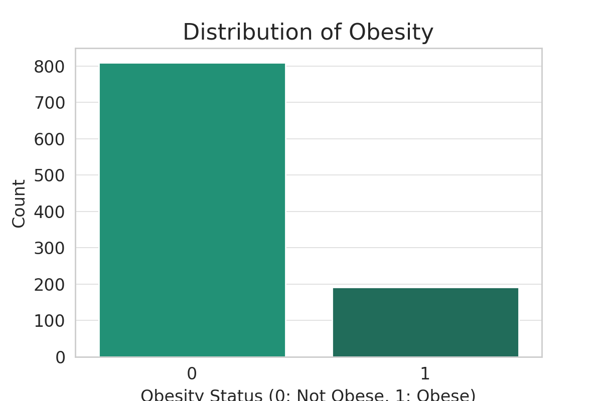
Let’s see the distribution of the obesity:
# Distribution of Obesity
plt.figure(figsize=(6, 4))
sns.countplot(x='Obesity', data=obesity_data)
plt.title('Distribution of Obesity')
plt.xlabel('Obesity Status (0: Not Obese, 1: Obese)')
plt.ylabel('Count')
Splitting the dataset
Before we build the logistic regression model in python environment, we’ll split the dataset into training and testing sets. This is an essential step to evaluate the model’s performance on unseen data, ensuring that our model can generalize well. We typically use around 70-80% of the data for training and the rest for testing. Let’s proceed with splitting the data.
from sklearn.model_selection import train_test_split

# Defining the features (X) and the target variable (y)
X = obesity_data.drop('Obesity', axis=1)
y = obesity_data['Obesity']

# Splitting the dataset into training (80%) and testing (20%) sets
X_train, X_test, y_train, y_test = train_test_split(X, y, test_size=0.2, random_state=42)

# Displaying the sizes of the training and testing sets to confirm the split
(X_train.shape, X_test.shape, y_train.shape, y_test.shape)
The dataset has been successfully split into training and testing sets, with the following sizes:

- Training set: 800 samples
- Testing set: 200 samples
This split ensures that we have a sufficient amount of data to train our model, as well as a separate dataset to evaluate its performance.
Model Building
Now, we’ll build a logistic regression model using the training data. First, We will fit the logistic regression model to the training data. Second , We will use the testing data to evaluate the model’s performance. Third, We will evaluate our model’s performance.
from sklearn.metrics import accuracy_score, confusion_matrix, classification_report

# Instantiate the logistic regression model
log_reg = LogisticRegression(max_iter=1000)

# Fit the model to the training data
log_reg.fit(X_train, y_train)

# Make predictions on the testing set
y_pred = log_reg.predict(X_test)

# Evaluate the model's performance
accuracy = accuracy_score(y_test, y_pred)
conf_matrix = confusion_matrix(y_test, y_pred)
class_report = classification_report(y_test, y_pred)

# Display the evaluation metrics
accuracy, conf_matrix, class_report
Our model achieved exceptionally accuracy of 99.5% on the testing set. In practical life it might be uncommon, however, we don’t know the true nature of the data. The dataset could be synthetic!(We don’t know!)
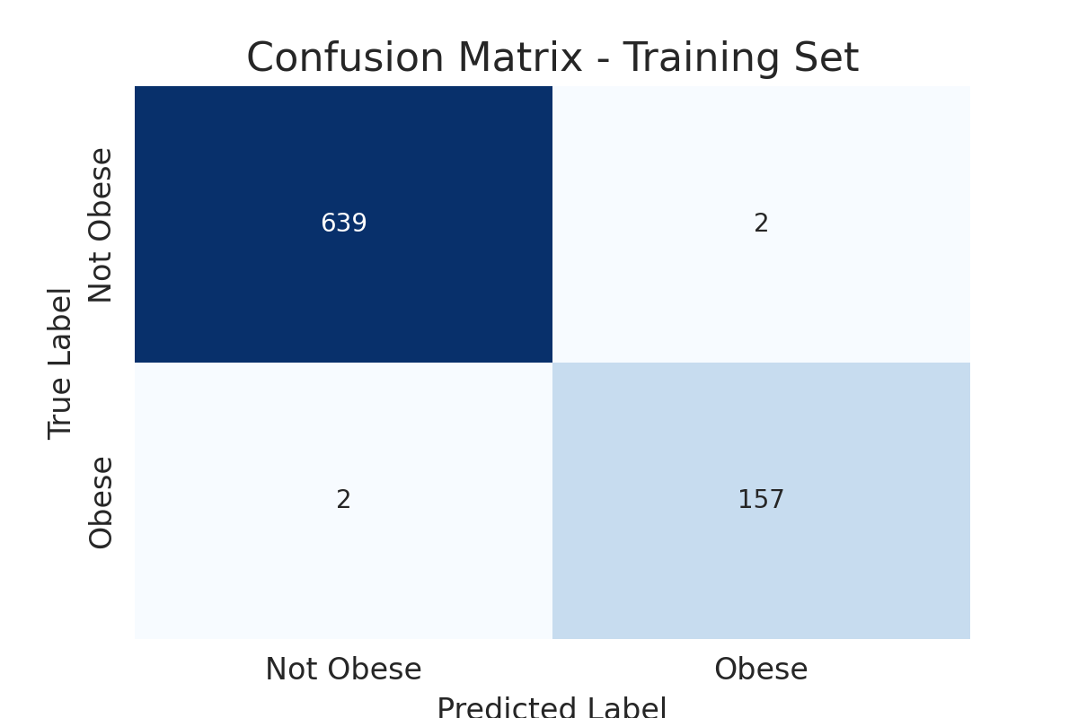
Now to see whether the models performance is truly valid, we run a confusion matrix
# Calculating confusion matrix for the training set
conf_matrix_train = confusion_matrix(y_train, y_train_pred)

conf_matrix_train
True Negatives (639): The model correctly predicted ‘Not Obese’ for 639 instances. False Positives (2): The model incorrectly predicted ‘Obese’ for 2 instances that were actually ‘Not Obese’. False Negatives (2): The model incorrectly predicted ‘Not Obese’ for 2 instances that were actually ‘Obese’. True Positives (157): The model correctly predicted ‘Obese’ for 157 instances.
Indeed, our confusion matrix results are consistent with our models performance: The model shows a strong ability to correctly classify both ‘Obese’ and ‘Not Obese’ instances, with very few errors. This supports the reliability of the 99% accuracy observed on the testing set.
A visual representation of confusion matrix